import geopandas as gpd
import numpy as np
import matplotlib.pyplot as plt
import pygeoda
from spatial_cluster_helper import ensure_datasets3 Multivariate Local Spatial Clusters
The detection of clusters using local indicators of spatial autocorrelation (LISA) statistics is arguably one of the most common applications of spatial data exploration. As argued in Chapter 18 of the GeoDa Explore Book, extending the familiar univariate measures like the Local Moran statistic to the multivariate domain is fraught with difficulties. The local neighbor match test, outlined in Anselin and Li (2020) and illustrated in Chapter 18 of the GeoDa Explore Book, is a new approach to visualize and quantify the trade-off between geographical and attribute similarity. The basic idea is to assess the extent of overlap between k-nearest neighbors in geographical space and k-nearest neighbors in multi-attribute space. This is illustrated with functionality from the specialized pygeoda package.
The local neighbor match test will be illustrated using the Chi-SDOH sample data set.
In addition to the pygeoda package mentioned, we will also need the familiar geopandas, numpy and matplotlib.pyplot packages, as well as spatial-cluster-helper to check on the presence of the sample data.
Required Packages
geopandas, numpy, matplotlib.pyplot, pygeoda, spatial-cluster-helper
Required Data Sets
Chi-SDOH
3.1 Preliminaries
3.1.1 Import Required Modules
We import the relevant modules.
3.1.2 Load Data
We use the same approach as in the previous Chapter and assume that the data are contained in a ./datasets/ directory off the main directory. We use ensure_datasets to load the sample data if not already present.
We read the Chi-SDOH.shp shape file into the chi_sdoh GeoDataFrame and provide a quick check of its contents.
# Setting data folder:
#path = "/your/path/to/data/"
path = "./datasets/"
# Select the Chicago census tract data:
shpfile = "Chi-SDOH/Chi-SDOH.shp"
# Load the data:
ensure_datasets(shpfile, folder_path = path)
chi_sdoh = gpd.read_file(path + shpfile)
print(chi_sdoh.shape)
print(chi_sdoh.head(3))
(791, 56)
OBJECTID Shape_Leng Shape_Area TRACTCE10 geoid10 commarea \
0 1 22777.477721 2.119089e+07 842400.0 1.703184e+10 44.0
1 2 16035.054986 8.947394e+06 840300.0 1.703184e+10 59.0
2 3 15186.400644 1.230614e+07 841100.0 1.703184e+10 34.0
ChldPvt14 EP_CROWD EP_UNINSUR EP_MINRTY ... ForclRt EP_MUNIT \
0 30.2 2.0 18.6 100.0 ... 0.0 6
1 38.9 4.8 25.2 85.9 ... 0.0 2
2 40.4 4.9 32.1 95.6 ... 0.0 42
EP_GROUPQ SchHP_Mi BrownF_Mi card cpval COORD_X COORD_Y \
0 0.0 0.323962 0.825032 0.0 0.0 1176.183467 1849.533205
1 0.0 2.913039 0.833580 0.0 0.0 1161.787888 1882.078567
2 0.1 1.534987 0.245875 0.0 0.0 1174.481923 1889.069999
geometry
0 POLYGON ((1177796.742 1847712.428, 1177805.261...
1 POLYGON ((1163591.927 1881471.238, 1163525.437...
2 POLYGON ((1176041.55 1889791.988, 1176042.377 ...
[3 rows x 56 columns]3.1.3 Variables
Following our standard practice, we specify the variable names to be used in the neighbor match test here.
For the neighbor match test example, we will use the percentage children in poverty in 2014 (ChldPvt14), a crowded housing index (EP_CROWD), and the percentage without health insurance (EP_UNINSUR). These are specified in the list nbrvars.
# Variables for neighbor match test:
nbrvars = ['ChldPvt14','EP_CROWD','EP_UNINSUR']
3.2 Local Neighbor Match Test
The Local Neighbor Match Test is based on an intersection operation between two k-nearest neighbor weights matrices. One matrix is derived from the distances in multi-attribute space, the other using geographical distance. With the intersection in hand, the probability that an overlap occurs between the two neighbor sets can be quantified. This corresponds to the probability of drawing \(v\) common neighbors from the \(k\) out of \(n−1−k\) possible choices as neighbors, a straightforward combinatorial calculation.
Specifically, the probability of \(v\) shared neighbors out of \(k\) is:
\(p=C(k,v).C(N−k,k−v)/C(N,k),\)
where \(N=n−1\) (one less than the number of observations), \(k\) is the number of nearest neighbors considered in the connectivity graphs, \(v\) is the number of neighbors in common, and \(C\) is the combinatorial operator. Details can be found in Chapter 18 of the GeoDa Explore Book.
The Local Neighbor Match Test is carried out by means of the neighbor_match_test function from pygeoda.
3.2.1 pygeoda Logic
The pygeoda package forms an interface between Python and a subset of the C++ code in GeoDa, contained in the libgeoda library. It implements basic data extraction functions, as well as the construction of spatial weights, computation of local spatial autocorrelation statistics and spatial clustering. The full API can be found at https://geodacenter.github.io/pygeoda/api.html.
pygeoda uses its own internal data structure, so before any analysis can be carried out, an existing DataFrame or GeoDataFrame must be loaded by means of the pygeoda.open command. After this step, variables are extracted in the same manner as for data frames, i.e., by specifying the variable name in quotes or as a list of quoted variable names. In our example, this will be the nbrvars list created in Section 3.1.3.
The return object of a pygeoda analysis is an instance of a specialized class, with a range of properties accessible as attributes. It is important to check the API for the specific structure in each function. The spatial_cluster_helper module used to check on the data set also contains a set of helper functions to simplify the extraction of results from the pygeoda return object. However, for the neighbor_match_test, this is not needed.
3.2.2 neighbor_match_test Function
The pygeoda.neighbor_match_test function has three required arguments:
geoda_obj(geoda): An instance of geoda classdata(list or dataframe): A list of numeric vectors of selected variable or a data frame of selected variablesk(int): A positive integer as the number of k-nearest neighbors.
In our example, the geoda_obj chi_sdoh_g will be created from the chi_sdoh GeoDataFrame using the open function, which converts it to a geoda class object. The list of variables is in nbrvars. The value of k is set to 12.
Additional optional arguments that can be provided to the function are:
scale_method(str, optional): One of the scaling methods (‘raw’, ‘standardize’, ‘demean’, ‘mad’, ‘range_standardize’, ‘range_adjust’) to apply on input data. Default is ‘standardize’ (Z-score normalization).distance_method(str, optional): The type of distance metric used to measure the distance between input data. Options are (‘euclidean’, ‘manhattan’). Default is ‘euclidean’.power(float, optional): The power used in an inverse distance calculation, default is 1.0.is_inverse(bool, optional): False (default) or True, apply inverse on distance value.is_arc(bool, optional): False (default) or True, compute arc distance between two observations.is_mile(bool, optional) True (default) or False, distance units used.
The function returns a dictionary with two keys: Cardinality and Probability. The cardinalities indicate for each location how many neighbors the two weights matrices have in common, whereas the probability shows the associated p-value. Different p-value cut-offs can be employed to select the significant locations, i.e., where the probability of a given number of common neighbors falls below the chosen p.
The example below consists of four steps:
- create the geoda data object
chi_sdoh_g - extract the variables into
data - return the result object to
nmt - print the
keysof the dictionary
chi_sdoh_g = pygeoda.open(chi_sdoh)
data = chi_sdoh_g[nbrvars]
nmt = pygeoda.neighbor_match_test(chi_sdoh_g, data, 12)
print(nmt.keys())
dict_keys(['Cardinality', 'Probability'])3.2.3 Neighbor Cardinality Map
We can now use matplotlib to create a categorical map to plot the neighbor cardinalities for each location. First, we need to add the Cardinality values to the existing chi_sdoh GeoDataFrame, to which we can then apply the plot functionality. We use the commands covered in Chapter 2 to set the column to Cardinality, specify the map type as categorical, and choose a color map, edgecolor and linewidth.
chi_sdoh['Cardinality'] = nmt['Cardinality']

fig, ax = plt.subplots(figsize = (6, 6))

chi_sdoh.plot(ax = ax,
              column = 'Cardinality',
              legend = True,
              categorical = True,
              cmap = 'YlOrRd',
              edgecolor = 'black',
              linewidth = 0.1)

ax.set_axis_off()
plt.show()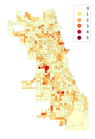
The matches range from 1 to 5 (out of a possible 12). There are three locations with four matches and two locations with five matches. Five matches is extremely rare, with a p-value less than 0.0000001. Four matches has a p-value less than 0.000014. These suggest locations of multivariate local spatial clusters.
3.3 Practice
Use your own data set or one of the GeoDa Center or PySAL sample data sets to load a multivariate data file. Compute the Local Neighbor Match Test and assess the impact of varying number of neighbors.