import numpy as np
import geopandas as gpd

from sklearn.cluster import KMeans
from sklearn.preprocessing import StandardScaler

from spatial_cluster_helper import ensure_datasets, cluster_stats, \
cluster_fit, cluster_map11 Spatializing Classic Clustering Methods
As such, the results of a classic clustering method like K-Means typically do not form spatially connected clusters, i.e., clusters for which the elements are spatially contiguous. In Chapter 12 and Chapter 13, we cover methods to impose hard spatial constraints to a clustering method. Here, we illustrate a way to impose soft spatial constraints, in the sense that the solution is nudged towards a spatially contiguous set, but this is not necessarily satisfied.
First, we show a simple regionalization method by applying a classic clustering method to the centroid coordinates of spatial units. We already illustrated an example of this for K-Medoids in Chapter 9. Here, we will apply K-Means to the centroid coordinates.
A second approach adds the centroid coordinates as additional features to the clustering procedure. This pushes the solution to a more spatially contiguous one, but it is only a soft constraint. In addition, the degree to which the nudging is effective depends on the number of other variables in the clustering exercise.
Further details are provided in Chapter 9 of the GeoDa Cluster Book. That Chapter also includes two additional methods that are primarily for pedagogical purposes to illustate the trade-offs involved in imposing spatial constraints. Since they are non-standard, they are not considered here.
To implement the spatialization, no new packages are required, since the methods are the same as before. The only changing element is the inclusion of coordinates among the features. Therefore, we again use StandardScaler from sklearn.preprocessing for variable standardization, as well as KMeans from sklearn.cluster to illustrate the effect on the cluster results. We also import the helper functions ensure_datasets, cluster_stats, cluster_fit and cluster_map from the spatial-cluster-helper package. Furthermore, we use numpy and geopandas.
The empirical illustration replicates the examples in Chapter 9 of the GeoDa Cluster Book with the ceara sample data set.
Required Packages
numpy, geopandas, sklearn.cluster, sklearn.preprocessing, spatial-cluster-helper
Required Data Sets
ceara
11.1 Preliminaries
11.1.1 Import Required Modules
11.1.2 Load Data
We read the data from the ceara.shp shape file and carry out a quick check of its contents. For this sample data, we use the argument encoding = 'utf-8' in the read_file function to account for the special characters in Brazilian Portuguese.
# Setting working folder:
#path = "/your/path/to/data/"
path = "./datasets/"
# Select the Ceará data:
shpfile = "ceara/ceara.shp"
# Load the data:
ensure_datasets(shpfile, folder_path = path)
dfs = gpd.read_file(path + shpfile, encoding = 'utf-8')
print(dfs.shape)
dfs.head(3)
(184, 36)| code7 | mun_name | state_init | area_km2 | state_code | micro_code | micro_name | inc_mic_4q | inc_zik_3q | inc_zik_2q | ... | gdp | pop | gdpcap | popdens | zik_1q | ziq_2q | ziq_3q | zika_d | mic_d | geometry | |
|---|---|---|---|---|---|---|---|---|---|---|---|---|---|---|---|---|---|---|---|---|---|
| 0 | 2300101.0 | Abaiara | CE | 180.833 | 23 | 23019 | 19ª Região Brejo Santo | 0.000000 | 0.0 | 0.00 | ... | 35974.0 | 10496.0 | 3.427 | 58.043 | 0.0 | 0.0 | 0.0 | 0.0 | 0.0 | POLYGON ((5433729.65 9186242.97, 5433688.546 9... |
| 1 | 2300150.0 | Acarape | CE | 130.002 | 23 | 23003 | 3ª Região Maracanaú | 6.380399 | 0.0 | 0.00 | ... | 68314.0 | 15338.0 | 4.454 | 117.983 | 0.0 | 0.0 | 0.0 | 0.0 | 1.0 | POLYGON ((5476916.288 9533405.667, 5476798.561... |
| 2 | 2300200.0 | Acaraú | CE | 842.471 | 23 | 23012 | 12ª Região Acaraú | 0.000000 | 0.0 | 1.63 | ... | 309490.0 | 57551.0 | 5.378 | 68.312 | 0.0 | 1.0 | 0.0 | 1.0 | 0.0 | POLYGON ((5294389.783 9689469.144, 5294494.499... |
3 rows × 36 columns
# the full set of variables
print(list(dfs.columns))
['code7', 'mun_name', 'state_init', 'area_km2', 'state_code', 'micro_code', 'micro_name', 'inc_mic_4q', 'inc_zik_3q', 'inc_zik_2q', 'inc_zik_1q', 'prim_care', 'ln_gdp', 'ln_pop', 'mobility', 'environ', 'housing', 'sanitation', 'infra', 'acu_zik_1q', 'acu_zik_2q', 'acu_zik_3q', 'pop_zikv', 'acu_mic_4q', 'pop_micro', 'lngdpcap', 'gdp', 'pop', 'gdpcap', 'popdens', 'zik_1q', 'ziq_2q', 'ziq_3q', 'zika_d', 'mic_d', 'geometry']11.1.3 Município Centroids
The locational coordinates are obtained as the centroids of the municípios.
As illustrated for K-Medoids in Chapter 9, we use the GeoPandas centroid attribute applied to our GeoDataFrame (dfs), then extract the x and y coordinates and add them as new variables. We rescale them by 1000 to keep the distance units manageable. Since the original coordinates are projected, it is appropriate to apply Euclidean distance.
cent = dfs.centroid
dfs['X'] = cent.x / 1000
dfs['Y'] = cent.y / 1000
11.1.4 Data Preparation
As customary, we compute the scaling factor nn for GeoDa compatibility. We also set the number of clusters to 12.
n = dfs.shape[0]
nn = np.sqrt((n - 1.0)/n)
n_clusters = 12
11.2 K-Means on Centroid Coordinates
We first illustrate a straightforward application of K-Means to the centroids of the municípios. We define data_cluster as a subset of the GeoDataFrame with just the coordinates and apply StandardScaler and the nn rescaling to create the input array X. Note that this runs counter to our earlier recommendation not to standardize coordinates. However, we use it here to keep the results comparable with the other clustering methods.
data_cluster = dfs[['X', 'Y']]
X0 = StandardScaler().fit_transform(data_cluster)
X = X0 * nn
We now apply KMeans with the usual arguments (see Chapter 8 for details) and obtain the cluster labels as labels_. We then apply cluster_stats, cluster_fit and cluster_map to characterize the results.
kmeans = KMeans(n_clusters = n_clusters, n_init = 150,
                init = 'k-means++', random_state = 123456789).fit(X)
cluster_labels = kmeans.labels_
c_stats = cluster_stats(cluster_labels)
clusfit = cluster_fit(data = data_cluster, clustlabels = cluster_labels,
                      correct = True, n_clusters = n_clusters)
Labels Cardinality
0 20
1 12
2 21
3 10
4 16
5 7
6 16
7 11
8 12
9 29
10 13
11 17
Total Sum of Squares (TSS): 366.0
Within-cluster Sum of Squares (WSS) for each cluster: [2.075 1.514 2.613 1.915 1.847 1.115 1.272 1.033 1.614 2.798 1.523 2.391]
Total Within-cluster Sum of Squares (WSS): 21.709
Between-cluster Sum of Squares (BSS): 344.291
Ratio of BSS to TSS: 0.941cluster_map(dfs, cluster_labels, figsize = (4,4),
cmap = 'Set3', title = "", legend_fontsize=8)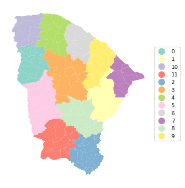
The results show a very nice regionalization, with good separation for BSS/TSS of 0.941. The resulting regions can then be used for data aggregation or as fixed effects variables in a spatial regression, among several other possibilities.
Similar results can be obtained by applying other classic clustering methods to the coordinates. This is not pursued further.
11.3 K-Means with Coordinates as Additional Features
A soft spatial constraint is introduced by adding the X-Y coordinates to the regular features. We illustrate this for K-Means.
We create two lists with cluster variables from the Ceará data set, following the example in Section 9.3.1. of the GeoDa Cluster Book. In the first list (clust_vars1), we include six socio-economic indicators: mobility, environ, housing, sanitation, infra, and gdpcap. The second list (clust_vars2) also contains X and Y.
clust_vars1 = ["mobility", "environ", "housing", "sanitation", "infra","gdpcap"]
clust_vars2 = clust_vars1 + ["X", "Y"]
11.3.1 K-Means with Features Only
We proceed in the by now familiar manner to create data_cluster1 as a subset of the GeoDataFrame, and apply the StandardScaler and the nn scaling factor to obtain the input matrix X. We then carry out KMeans with the usual arguments and summarize the results by means of our helper functions.
data_cluster1 = dfs[clust_vars1]
X0 = StandardScaler().fit_transform(data_cluster1)
X = X0 * nn
kmeans = KMeans(n_clusters = n_clusters, n_init = 150,
init = 'k-means++', random_state=123456789).fit(X)
cluster_labels1 = kmeans.labels_
c_stats = cluster_stats(cluster_labels1)
clusfit = cluster_fit(data = data_cluster1, clustlabels = cluster_labels1,
correct = True, n_clusters = n_clusters) Labels Cardinality
0 21
1 30
2 3
3 22
4 4
5 10
6 7
7 1
8 23
9 26
10 26
11 11
Total Sum of Squares (TSS): 1098.0
Within-cluster Sum of Squares (WSS) for each cluster: [35.969 37.901 5.341 43.958 11.088 27.469 27.094 0. 38.359 46.621
51.678 22.647]
Total Within-cluster Sum of Squares (WSS): 348.125
Between-cluster Sum of Squares (BSS): 749.875
Ratio of BSS to TSS: 0.683cluster_map(dfs, cluster_labels1, figsize = (4,4),
cmap = 'Set3', title = "", legend_fontsize=8)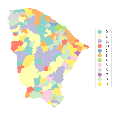
The clusters are not identical to the solution obtained with GeoDa, but the results are close. The fit is quite good, with a BSS/TSS ratio of 0.683. However, there is very little spatial clustering. Cluster 4 is the only one that turns out to be spatially contiguous, consisting of 4 municípios surrounding the main city of Fortaleza. However, in contrast, for cluster 7, which also consists of 4 units, the four entities are totally disconnected in space.
11.3.2 K-Means with X-Y Included as Features
We now include the X and Y coordinates among the features using clust_vars2 as the input, but otherwise we proceed in exactly the same way as before.
data_cluster2 = dfs[clust_vars2]
X0 = StandardScaler().fit_transform(data_cluster2)
X = X0 * nn
kmeans = KMeans(n_clusters = n_clusters, n_init = 150,
init = 'k-means++', random_state = 123456789).fit(X)
cluster_labels2 = kmeans.labels_
c_stats = cluster_stats(cluster_labels2)
clusfit = cluster_fit(data = data_cluster2, clustlabels = cluster_labels2,
correct = True, n_clusters = n_clusters) Labels Cardinality
0 30
1 15
2 9
3 15
4 3
5 17
6 19
7 15
8 13
9 24
10 4
11 20
Total Sum of Squares (TSS): 1464.0
Within-cluster Sum of Squares (WSS) for each cluster: [93.898 28.392 51.527 57.266 14.62 38.063 49.986 49.473 45.144 64.804
11.152 52.565]
Total Within-cluster Sum of Squares (WSS): 556.891
Between-cluster Sum of Squares (BSS): 907.109
Ratio of BSS to TSS: 0.62cluster_map(dfs, cluster_labels2, figsize = (4,4),
cmap = 'Set3', title = "", legend_fontsize=8)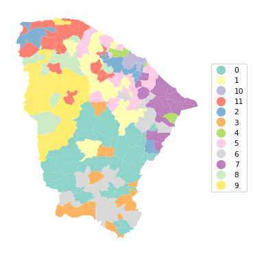
The results show more of a spatial grouping, although the solution is by no means fully contiguous. The price we pay for the inclusion of the coordinates is a decline of BSS/TSS to 0.62.
11.4 Practice
It is straightforward to include X-Y coordinates into the cluster analyses carried out in the previous Chapters. Assess the extent to which this creates more spatially contiguous cluster results.